For the final project of the course 16-782 Planning and Decision-Making in Robotics course at Carnegie Mellon University, I worked in a team to develop an approach that can be utilized for solving planning involving granular materials through the use of the weighted A* search algorithm. We tested our approach on a planar robot wiping task that aims to move a collection of cylinders into a goal region while optimizing for the total number of actions taken in the plan. The transition model we use to model collisions between the objects in the environment and the robot uses the PyBullet simulator for state estimation and to determine the resulting dynamics of the collisions. Additionally, our transition model consists of a less computationally expensive free space motion transition model to increase performance. Our method was able to successfully produce plans for a variety of environment configurations.
The code for our project can be found as a Github repository here.
Approach
A simulator is used to model the physical interactions between objects. Our robot, which is a planar pusher, uses a predefined urdf composed of two prismatic joints and one revolute joint to move itself on a plane. A block is modeled as a small cylinder, which is also loaded through an urdf. The blocks can move freely along the plane, while the robot has a heading direction. Initially, one robot and N blocks are placed on a table. There are predefined goal areas on the table. When a block reaches any of the goal areas, it falls off the table. The task is to control the robot to push all blocks off the table.

Planning Algorithm
We implement the planner in Python; Numpy, Shapely, and PyBullet are the three main external libraries we use. The real world states from the simulator are continuous, while the weighted A* algorithm works on discrete states. Quantization and inverse quantization are used to translate state representations between simulator and graph. Specifically,

where q_d and q_a are quantization steps for location on the plane and the heading, respectively. x, y, and θ represent the states in the graph, while X, Y and Θ represent the states in the simulator.
We use an implicit graph for the planner. An implicit graph is chosen since we cannot assume that either the robot’s state or the blocks’ states after an action lie directly in the discretized states. Additionally, the search space of this task is large; the dimension of the planning space is equal to 3 + 2N, where 3 comes from the robot state and 2N comes from the block states. Each node in the graph stores both the robot state S_R(x, y, θ) and the world state (S_B(x_1, y_1), ··· , SB(x_N, y_N)), as well as the standard fields in weighted A*, such as the cost-from-start g and heuristics h. We implement the implicit graph, where the nodes are stored, in a vector. We utilize a look up table (as a dictionary) for querying a node’s existence in the graph. The key of the dictionary is the concatenation of the robot and world state. The value of the dictionary is the index to the node vector.
Heuristics
We wanted to encourage the blocks to be near the goal region, which can be achieved by penalizing the sum or max of each block’s distance to its nearest goal cell. To guarantee ε optimality, we can use the longest K distance as the heuristic when the number of blocks becomes large. However, when the robot is far from the blocks, the robot will search uniformly through a large high dimensional sphere. To avoid this, we add another heuristic that represents the distance from the robot to the blocks. A reasonable implementation of this idea is to check the distance between the robot and the block that has the furthest distance to its nearest goal cell.
Speedups
To simplify our algorithm in terms of speed and computation, we introduce a free space motion model. For each action during planning, we first use a shape based free space motion model to check for collisions between the robot and blocks. If so, we call the simulator to calculate the robot and world state after the collision. Otherwise, we bypass the simulator and use the free space motion model’s robot state as the new robot state while keeping the world state unchanged.
Results
We conducted various experiments to examine the completeness and robustness of our model. The experiments focused on the planning time of the A* algorithm, the performance of the different heuristic components, the number of steps to arrive to the goal (all blocks in goal area), and the free space transitions.
To test the factors mentioned above, we used two testing methods: generating specific scenarios and a randomized method. The specific scenarios we tested were of easy, medium and more difficult configurations. In easier configurations the robot was placed very close to the block(s) and we usually tested a small number of blocks, such as one or two. The medium configurations would be a bit further apart and slightly trickier–say the robot was placed near one corner of the goal, one block across the goal, and a different block in the opposite direction from the robot. The difficult configurations would include more blocks and dispersed through the map.
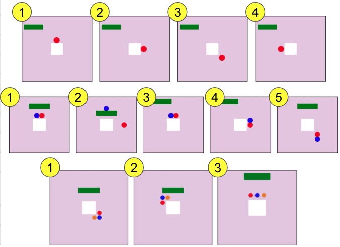
The two videos below show two different examples of the planner, one with three beads and the pusher starting far away, and the second with six beads but the pusher much closer.
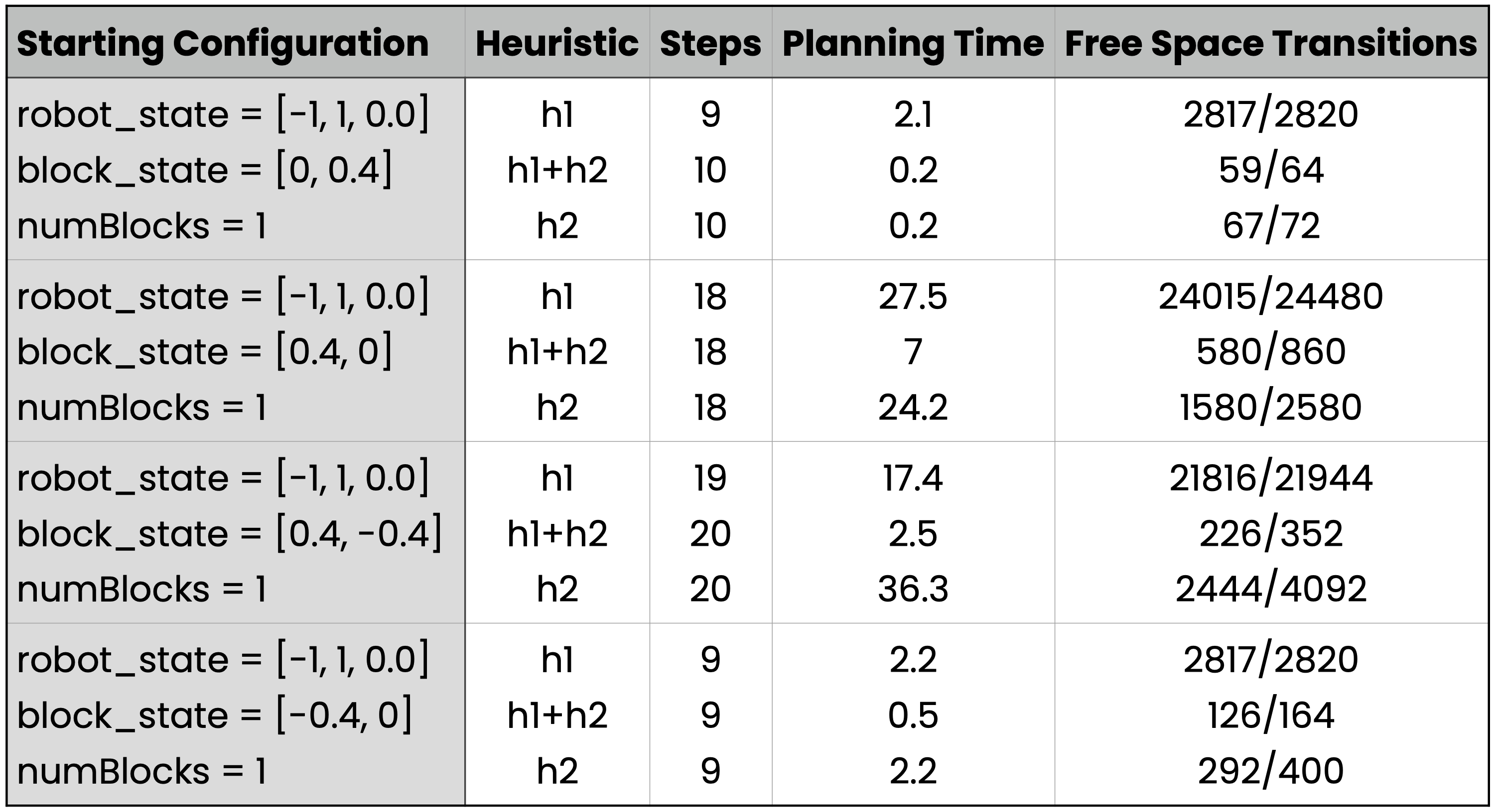
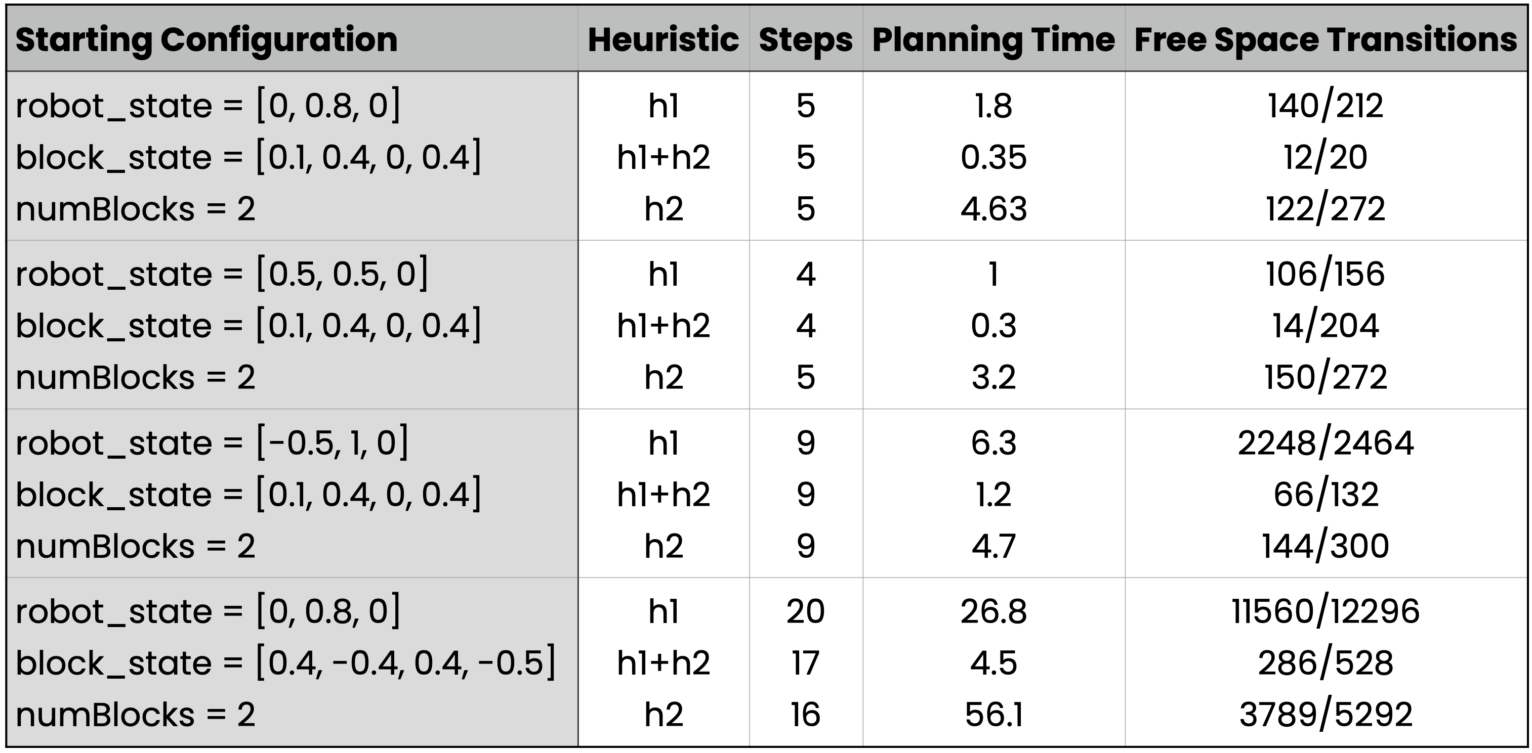
By running these various tests and parsing through the results, we were able to discern what factors positively contributed to our heuristics or what difficulties the planner encountered for repeated starting configurations. Some of our results can be seen in Table 1 and Table 2, for one and two blocks, for comparison between our two heuristics alone, and their cumulative results. We can see from these results that the combination of both heuristics outperform any singular performance.
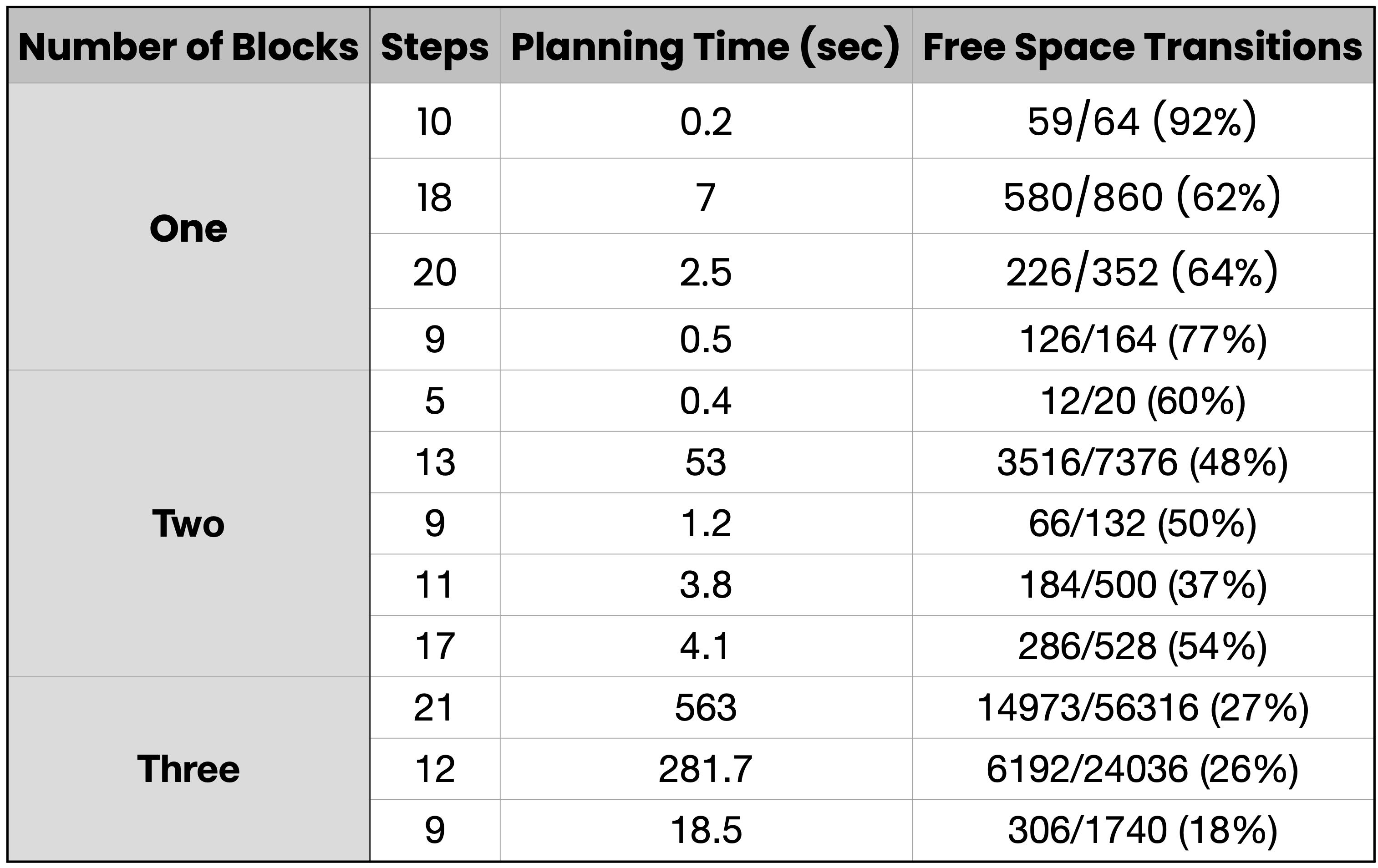
The random configurations we used require a number of blocks to be selected and then it randomizes the starting position of the blocks and the starting position and orientation of the robot. These experiments allowed us to test and verify completeness of our planner and model with random configurations repeatedly. It proved to be a valuable analysis tool as, even though planning took a long time for some scattered starting configurations, we validated our algorithms for more than our hard-coded set of starting configurations.
For testing the randomized configurations, we used the combined heuristics for all the tests. Results for various random configurations with one, two and three blocks are shown below with the results shown in Table 3.